
This is article 5 in a series on VTK. The first in this series can be found here. We discuss creating lookup tables that map model data to the colours that appear on models in visualisations.
In the last section a lookup table was used to colour polygons based on cell and node data. If you are unfamiliar with colour formats you may want to read this article on colour models for more information.
Colour can be very useful to convey information in visualisations. To set a single colour for an actor, you can use the actor.GetProperty().SetColor(r, g, b) command. This will set the entire model to a single colour defined by the (r, g, b) values provided.
For scientific visualisations you will want to draw objects in different colours to communicate information about the data associated with the model. In VTK the lookup table is the object that maps scalar values to colours. The analyst modifies the lookup table to adjust the colour scheme or otherwise control how scalar values are mapped to colours to represent data.
A lookup table for polygon data is created using lut = vtk.vtkPolyDataMapper(). The lookup table is associated with a model through the mapper object. The method .SetLookupTable(lut) connects the lookup table lut to the mapper. Further, the method .SetUseLookupTableScalarRange(True) needs to be called on the mapper. This causes the mapper to use the same range as that used by the lookup table. Not using this method will cause the mapper to override the range set in the lookup table which is probably not what you want.
No matter the parameters used in a lookup table, it is necessary to call the .Build() method. This updates the lookup table to reflect the updated settings.
We continue in the next example showing how to achieve different results by tweaking lookup table settings.
Default lookup tables
By default a lookup table will use the rainbow range of colours which often appear on scientific visualisations. These colours are approximately red, yellow, green, aqua, blue, with red mapped to the lower end of the table’s range and blue at the upper end.
The range for a lookup table is set with the method .SetTableRange(low, high). By default values above or below this range will be shown with the same colour as the nearest value in the range, e.g., a value of 400 for a table with range [500, 600] would have the same colour as a value of 500. It is possible to set custom colours for values outside the range using the methods .SetAboveRangeColor(colour) and .SetBelowRangeColor(colour). Here colour is a list of 4 values, the usual 3 RGB values plus an alpha channel. No matter whether one or both of these methods have been called, it is possible to control whether this feature—using a custom colour for values outside the range—is activated with these 4 methods:
-
.UseBelowRangeColorOn() -
.UseBelowRangeColorOff() -
.UseAboveRangeColorOn() -
.UseAboveRangeColorOff()
The feature is off by default so must be activated.
Custom colour ranges for gradients
Although the default rainbow colour scheme is useful in most cases, it is possible to customise how colours are mapped. This can be done by constraining the range for hue, saturation, or value of the resulting colours. The methods for this are:
-
.SetHueRange(low, high) -
.SetSaturationRange(low, high) -
.SetValueRange(low, high)
If low and high are the same value the corresponding parameter is fixed and does not vary with input data.
Different effects can be created by fixing some of the 3 parameters of the HSV model while allowing others to vary. By default the saturation and value are fixed at the maximum of 1.0 while the hue varies with input data. The result is the rainbow colour gradient described above.
The example below creates a greyscale colour map that varies with input value. The hue is fixed at an arbitrary number, the saturation is set to 0.0, and the value varies.
lut.SetHueRange(0.5, 0.5)
lut.SetSaturationRange(0.0, 0.0)
lut.SetValueRange(0.25, 1.0)
Creating arbitrary colour mappings
The previous examples have set parameters on the default lookup table provided by VTK. The first was the default rainbow lookup table. The second modified the ranges of the 3 HSV parameters to provide a particular greyscale effect.
VTK allows complete control over the lookup table. You can create any arbitrary mapping of values to colours. This requires individually specifying each mapping from value → colour.
Each lookup table has a fixed number of colours. This is set by the method .SetNumberOfColors(number) for an integer value number. The default is 256. This maps 256 colours across the range specified by .SetTableRange(low, high). Values are equally spaces for the default rainbow visualisation; however, any arbitrary scale can be set.
Once the number of colours in a lookup table has been set, the individual mappings are set with the method .SetTableValue(id, R, G, B, A). The parameters R, G, and B specify the colour to which a data value maps. The alpha channel is specified by A. The optional parameter A defaults to 1.0 if not specified, i.e., .SetTableValue() is called with just 4 parameters. The id is an integer that specifies where within the range this colour sits. If \$N\$ colours are used in a table then id varies from 0 to \$(N-1)\$. A value below or above the range will map to the colours with id 0 or \$N-1\$ respectively.
Displaying categorical data
Arbitrary mappings between values and colours can be used to represent categorical information. This could be material damage in a mechanical simulation or healthy/unhealthy material in a medical scan.
To visualise categorical data we simply assign an arbitrary value between 0 and 1 to each category. We set the number of categories we need. For \$N\$ categories of data we set .SetNumberOfColors(N) and each category is set an arbitrary value for results in its category. For an example consider 4 categories these would have values of 0.0, 0.3333, 0.6666, and 1.0. If we allocate these categories an integer category number, cat_no, then the first category has cat_no = 0 and all cells of this category have a scalar cell value of 0.0. The second category has cat_no = 1 and cell value of 0.3333, and so on. Each category is then set its own colour using .SetTableValue(cat_no, R, G, B).
Creating custom colour gradients
The previous examples showed how colour gradients can be controlled by manipulating the ranges used across the HSV colour model when mapping data. The colours and their order is fixed. These include red, yellow, green, blue, and others. We can cut off this range of colours at either end by specifying a range for the hue. This was shown above.
What has not been shown is a method to create arbitrary colour gradients. Here by arbitrary colour gradients we want to be able to specify several intermediate colours and to create smooth colour gradients between those colours.
With VTK we instead we need to manually calculate the RGB values for each individual shade in the colour gradient and add this to the lookup table. There is no method to do this, but there are objects that can help.
VTK provides an object, vtkColorTransferFunction, to use when creating this lookup table. We use the method .AddRGBPoint(value, R, G, B) which takes 4 parameters. These are the value and a colour, specified using RGB values. Once these value-colour pairs have been set the method .GetColor(value) can be queried. For an arbitrary value it returns a colour which has been interpolated from the colours with the nearest value.
To illustrate, below is a vtkColorTransferFunction with yellow (RGB: 1.0, 1.0, 0.0) set to the value 0.0 and red (RGB: 1.0, 0.0, 0.0) set to 1.0. The colour orange (RGB: 1.0, 0.5, 0.0) is the colour half way between these two. Its RGB values are correctly returned when .GetColor(value) is called with a value of 0.5.
ctransfer = vtk.vtkColorTransferFunction()
ctransfer.AddRGBPoint(0.0, 1.0, 1.0, 0.0) # Yellow
ctransfer.AddRGBPoint(1.0, 1.0, 0.0, 0.0) # Red
# Correctly outputs the colour orange.
ctransfer.GetColor(0.5) # (1.0, 0.5, 0.0)
Once we create the vtkColorTransferFunction we set each individual colour in the lookup table. We need to generate the 256 individual colours that provide a smooth gradient.
We populate a lookup table below of \$N\$ evenly stepped values from \$a\$ to \$b\$. The value at position i from 0 to N is given by \$i \times \frac{b-a}{N}\$.
lut = vtk.vtkLookupTable()
lut.SetTableRange(a, b)
for i in range(N):
    new_colour = ctransfer.GetColor( (i * ((b-a)/N) ) )
    lut.SetTableValue(i, *new_colour)
lut.Build()
Example: Creating custom lookup tables
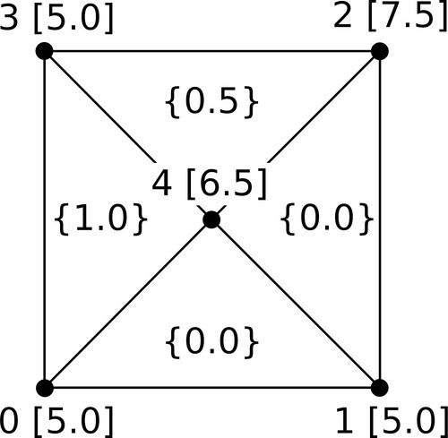
An example mesh of 4 cells and 5 nodes is used to display different visualisations of the same data with different lookup tables. The mesh has both scalar cell and node data. Values are shown in the example mesh. If both cell and node data are present in the model VTK defaults to visualising the node data.
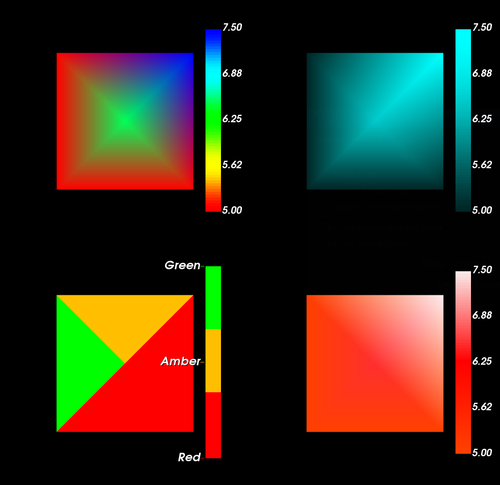
Four different lookup tables were created to visualise the data from the example mesh. The final results are shown below.
Only one mesh was created using an instance of vtkpolyData. The different visualisations are created using four different lookup tables, numbered 1 to 4 in the listings below. These correspond to the results below moving clockwise from the top-left.
The table ranges were set using:
lut_1.SetTableRange(5.0, 7.5)
lut_2.SetTableRange(5.0, 7.5)
lut_3.SetTableRange(5.0, 7.5)
lut_4.SetTableRange(0.0, 1.0)
The data ranges are set appropriately for the visualised data. The 4th example visualises category data set to the cells of the mesh.
For the first lookup table only the .Build() method was called before being assigned to the corresponding mapper.
lut_1.Build()
mesh_mapper_1.SetLookupTable(lut_1)
The second lookup table creates a blue, monochrome gradient in which the magnitude of input data corresponds to darker or brighter locations. This works well for 2D models. The use of shading on 3D models may distort the visualisation by darkening parts of the model to provide shadows and graphical fidelity rather than accurately reflecting the magnitude of the visualised data.
lut_2.SetHueRange(0.5, 0.5)
lut_2.SetSaturationRange(1.0, 1.0)
lut_2.SetValueRange(0.25, 1.0)
lut_2.Build()
mesh_mapper_2.SetLookupTable(lut_2)
The third lookup table creates a custom combination of colours from which smooth gradients are generated. This is generated using the method described above. Three colours are selected. They are set to reflect values at the low, middle, and high end of the value range. A vtkColorTransferFunction is used to interpolate the colour values to create a gradient between these three points.
no_of_colours = 256
lut_3.SetNumberOfColors(no_of_colours)

ctransfer = vtk.vtkColorTransferFunction()
ctransfer.AddRGBPoint(0.0, 1.0, 0.25, 0.0) # Orange
ctransfer.AddRGBPoint(0.5, 1.0, 0.00, 0.0) # Red
ctransfer.AddRGBPoint(1.0, 1.0, 0.95, 0.95) # White

for i in range(no_of_colours):
    new_colour = ctransfer.GetColor(i / float(no_of_colours))
    lut_3.SetTableValue(i, *new_colour)

lut_3.Build()
mesh_mapper_3.SetLookupTable(lut_3)
The final lookup table uses 3 custom colours to display membership of each cell in one of 3 categories. The number of colours is set to 3 with lut_4.SetNumberOfColors(3) and each of the 3 colours are set individually in the lookup table. The visualisation displays red, amber, or green for cell values 0.0, 0.5, or 1.0.
Note from the example mesh that this example includes both cell and node data. It was noted above that VTK defaults to displaying node data when both are provided. This can be overridden using the methods .SetScalarModeToUseCellData() and .SetScalarModeToUsePointData(). The latter is usually unnecessary as it is the default behaviour for VTK.
lut_4.SetNumberOfColors(3)
lut_4.SetTableValue(0, 1.0, 0.0, 0.0) # Red
lut_4.SetTableValue(1, 1.0, 0.75, 0.0) # Amber
lut_4.SetTableValue(2, 0.0, 1.0, 0.0) # Green

lut_4.Build()
mesh_mapper_4.SetLookupTable(lut_4)
mesh_mapper_4.SetScalarModeToUseCellData()
An instance of vtkScalarBarActor was added to each renderer. It helps to annotate a visualisation by providing a legend for colours and the values to which they correspond.
The precise cell value may not be useful for categorical information if it is arbitrary and only used to assign membership to a category. The default labels were removed from the scalar bar by setting their number to 0 with the method .SetNumberOfLabels(0) on the vtkScalarBarActor bar_4. Annotations were manually added using the lookup table method .SetAnnotation(value, annotation).
lut_4.SetAnnotation(0.0, "Red")
lut_4.SetAnnotation(0.5, "Amber")
lut_4.SetAnnotation(1.0, "Green")
Bars are assicated with a corresponding lookup table using bar.SetLookupTable(lut) and added to a renderer as an actor. Being a 2D actor they are added using the method .AddActor2D(actor).
All 4 results are shown in the results below.
Continue here for a description of how to transform and manipulate the position and geometry of a visualisation’s models.