
This is article 4 in a series on VTK. The first in this series can be found here. We discuss data models used in VTK and create polygon data with a simple triangle example.
The VTK pipeline begins with one or multiple data sources. This data is the result of experiments, calculations, or other measurements from the real world. There are different data structures that VTK offers which you can use to store your data. They have advantages with how much—or little—information needs to be provided to completely describe your data.
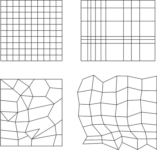
The more structured your numerical data the more that VTK can assume about the underlying geometry and the less that needs to be provided. The figure above shows data at 4 different levels of structure. In order of most to least structure, these are: image, rectilinear grid, structured grid, and polygonal data.
To fully describe image data you only need to provide:
-
The origin of the grid. This is a position vector that points to the corner of the grid with the lowest
x,y,zcoordinate values. These are 3 scalar values. -
The pitch between cells: This is a single scalar value and it describes the size (width) of all cells.
-
The dimensions of the image data. These are 3 scalar values,
l×m×n, which describe the number of cells in each dimension. One or more of these values are set to 1 for 1D or 2D image data.
The rectilinear grid requires more information to fully define it. The same information as an image is required, along with the pitch between each row of nodes: this is a single scalar value for each row. Note from the figure above cells are parallel, but the width of any cell is different for each row. This distance must be specified for each row.
The amount of information then increases further for the other data structures.
The type of data structure to use depends on the data that it will represent. It should be the most structured data which accurately represents the visualised geometry. Image data from a camera could be represented by a VTK image object, whereas a polygon mesh imported from a CAD programme would need to be represented by unstructured polygon data.
Using and creating polydata
In the previous example a polygon mesh was created from the cone source object. This was put through the pipeline and rendered without any further modification. In the following example a simple polygon mesh is created by manually specifying the location of each point. The connectivity between points is then specified to create a cell. Each mesh contains just one triangular cell.
Scientific visualisations feature geometry and a field of data assigned to points on that geometry. With a mesh of polygons used to represent that geometry the data values may be mapped to either the nodes or across entire cells of a mesh. A heatmap of scalar values across a geometry is such an example. VTK lets you create an array of values that map to either the points or cells in a mesh.
This time we also assign data values to the mesh. One mesh has a single data value assigned to the cell whereas the other has values assigned to the nodes of that cell.

points = vtk.vtkPoints()
cell = vtk.vtkCellArray()
mesh_1 = vtk.vtkPolyData()
mesh_2 = vtk.vtkPolyData()
tri = vtk.vtkTriangle()
Above we see the objects that are used to generate the polygon mesh geometry. These are composed together to create the final mesh. The result will be two vtkPolyData meshes of a single triangle, where the geometry of that triangle is referenced by both meshes.
# The first point will have a default ID of 0.
points.InsertNextPoint( (0.0, 0.0, 0.0) )
points.InsertNextPoint( (0.0, 1.0, 0.0) )
points.InsertNextPoint( (1.0, 0.0, 0.0) )
Above we see an instance of vtkPoints with data appended via the .InsertNextPoint() method. All points are also allocated an ID number incrementally from 0 in the order in which they were inserted. An alternative is to use the method .SetNumberOfPoints(numPoints) where numPoints is the number of points that will be stored. Individual points are then set using .SetPoint(id, (x, y, z) ). Importantly id cannot exceed 1 less than the value used as numPoints in the previous command, i.e., numPoints - 1. Exceeding the maximum allowable ID number, or setting a point .SetPoint() before memory is first allocated by first calling .SetNumberOfPoints(), will cause errors.
When .InsertNextPoint() is called, new memory in RAM is allocated for the new point. Similarly, the space necessary to store numPoints is allocated when .SetNumberOfPoints() is called. Other classes are similar in that the dimensions of a structure must first be specified after which individual items can be added to that structure, up to the number that was specified. If values are appended their ID is automatically set.
A triangle has 3 points. It is necessary to match global point IDs to the three points of the triangle. Points are matched using .GetPointIds().SetId(i, j). In our current example we used the same value for i and j because this example only features a single triangle polygon. The first value is one of 0, 1, or 2 and specifies the triangle’s local point ID. The second can be any global point ID. These are the IDs that were automatically allocated to nodes using .InsertNextPoint() or explicitly when calling .SetPoint() on an instance of vtkPoints.
for i in range(3):
    tri.GetPointIds().SetId(i, i)

cell.InsertNextCell(tri)
Objects in VTK are often composed of many smaller objects. Parameters/properties are often set by getting the relevant object from the larger object into which it is composed and setting that parameter. Here the triangle is composed of multiple points. .GetPointIds() returns a vtkIdList object on which we then call the .SetId() method.
Polygons are oriented. Orientation is determined by the right-hand rule and the position of the 3 global point IDs for the mesh.
Points and cells are then set to a mesh.
mesh_1.SetPoints(points)
mesh_1.SetPolys(cell)
We set the cell data for mesh_1. These scalar values are stored as double precision floating point values, which are suitable for most cases.
cell_data = vtk.vtkDoubleArray()
cell_data.SetNumberOfComponents(1)
cell_data.InsertNextTuple([0.5])
mesh_1.GetCellData().SetScalars(cell_data)
The array is first created, then the number of components are set. Regular scalar data will have 1 component, vectors will use 3 components and higher order tensors will use more. Data, even for scalars, is entered using a list. To enter vector quantities with three components the number of components needs to be set to 3 with .SetNumberOfComponents(3) and the one component list is replaced with a list of three quantities.
The last line assigns the data to the mesh itself. The order in which data is inserted into the vtkDoubleArray corresponds to how that data will line up with each cell in a mesh. Here the first (and only) tuple value added into the array corresponds with the first (and only) cell added to mesh_1. The process shown below is similar, but sets point data to the three points in the triangle.
point_data.InsertNextTuple([0.0])
point_data.InsertNextTuple([1.0])
point_data.InsertNextTuple([0.5])
mesh_2.GetPointData().SetScalars(point_data)
The rest of this code example is boilerplate, essentially unchanged from the previous example. An exception is the construction of the lookuptable. Lookuptables are discussed in the next section. A lookuptable assigns colours to numerical values.
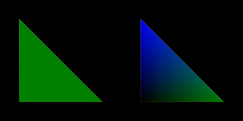
From the figure above we see the single coloured cell on the left. Here the cell’s scalar value maps to a single colour. On the right the cell is filled with linear gradients of colours. Colours are selected using the scalar values at the nodes, then gradients between these fill the contents of the cell.
Continue here for a description of how to map model data to colours that can be used to efficiently share information to the user of a visualisation.